Differential-Equation Models

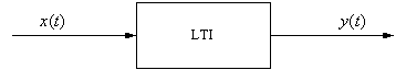
An important class of continuous time LTI systems are those modeled by ordinary linear differential equations with constant coefficients.

Given an input x(t) and an output y(t),

is a linear first-order (the order of the derivatives is one) differential equation with constant coefficients (as long as a and b are constants).

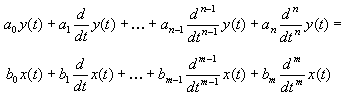
A general nth order linear differential equation with constant coefficients is:

which we can write as:

Solution of Differential Equations

A classical method for the solution of our differential equation is called the method of undetermined coefficients. We express the output y(t) as the sum of complementary or natural (y_c(t)) and particular or forced (y_p(t)) solutions:

y(t) = y_c(t) + y_p(t)

Natural response The natural response y_c(t) is the solution to the homogeneous equation:

Assume that the solution of the homogeneous equation is:

y_c(t)= Ce^st

Substituting in the homogeneous equation yields:

and we get:

This is the characteristic equation and it may be factored as:

The solution is of the form:

assuming there are no repeated roots (which is all we will cover here).

Ex.  Given a first-order differential equation

find its homogeneous solution. Your answer should be in terms of a constant C.

Forced response The forced response y_p(t) solves the equation

The form of the solution is determined by the input x(t). For an exponential input x(t)= A e^at, the solution would be y_p(t) = P e^at where A, a, and P are constants.

Ex.  For the previous example, assume an input x(t) = 6 e^{3 t}. Find the particular solution y_p(t).

Ex.  Now, assuming that the system is initially at rest (the initial conditions are 0), i.e., y(0) = 0 , solve for the constant C in your overall solution y(t) = y_c(t) + y_p(t):

Ex.  Given

y '(t) + 2y(t) = x(t)

where x(t) = 4 e^2t, find y(t). Assume y(0) = 0.