
In this lesson, we will discuss sampling of continuous time signals. Sampling a continuous time signal is used, for example, in A/D conversion, such as would be done in digitizing music for storage on a CD, digitizing a movie for storage on a DVD, or taking a digital picture.
To start, we define the continuous time impulse train as:

As you just saw, p(t) is an infinite train of continuous time impulse functions, spaced Ts seconds apart.
Now, x(t) is the continuous time signal we wish to sample. We will model sampling as multiplying a signal by p(t). Let xs(t) = x(t)p(t) be the sampled signal. Then

Let's show this graphically:
Now, we will derive the Sampling Theorem . To do this, we will examine our signals in the frequency domain. To start, let p(t) have a Fourier Transform P(ω), x(t) have a Fourier Transform X(ω), and xs(t) have a Fourier Transform Xs(ω).
Then, because xs(t) = x(t)p(t), by the Multiplication Property,
![]()
Now let's find the Fourier Transform of p(t). Because the infinite impulse train is periodic, we will use the Fourier Transform of periodic signals:

where Ck are the Fourier Series coefficients of the periodic signal.
Let's find the Fourier Series coefficients Ck for the periodic impulse train p(t):
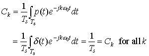
by the sifting property. Therefore
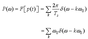
![]()
Thus, an impulse train in time has a Fourier Transform that is a impulse train in frequency. The spacing between impulses in time is Ts, and the spacing between impulses in frequency is ω0 = 2π/Ts. We see that if we increase the spacing in time between impulses, this will decrease the spacing between impulses in frequency, and vice versa. This is a very important result!
Now, to finish our derivation of the Sampling Theorem, we will go back and determine Xs(ω).
We saw that:

Therefore,

or we get replicated, scaled versions of X(ω), spaced every ω0 apart in frequency:
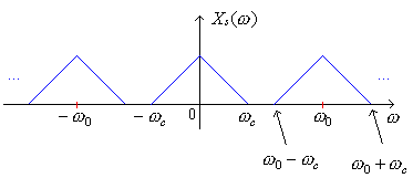
As you can see from the figure if ω0 - ωc < ωc, we would get overlap of the replicates of X(ω) in frequency. This is known as "aliasing." Therefore, to avoid aliasing, we require ω0 - ωc > ωc or ω0 > 2ωc. If we avoid aliasing, we can recover x(t) from its samples. (Usually, we choose a sampling rate a bit higher than twice the highest frequency since filters are not ideal.)
We hear music up to 20 kHz and CD sampling rate is 44.1 kHz. (Dogs would need a higher quality CD since they hear higher frequencies than humans.)
We can recover x(t) from its sampled version xs (t) by using a low pass filter to recover the center island:
Example 1 Given a signal x(t) with Fourier Transform with cutoff frequency ωc as shown:
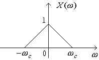
you are given three different pulse trains with periods
 |
, |  |
, and |  |
, |
draw the sampled spectrum in each case. Which case(s) experiences aliasing?
Example 2 The inverse Fourier Transform of the signal in the previous example is

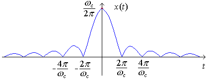
Draw the sampled signals using the sampling trains of the previous example
| ( |  |
, |  |
, and |  |
). |
Notice how aliasing looks in the time domain.
 |
 |
 |
 |
 |
 |
 |
 |
 |