![]()
M/M/1/K
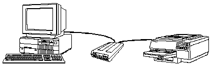
Example: Printer Buffer
![]()
Let's
look at a simple example of an M/M/1/K queuing system. One such example is a
printer buffer. These buffers sit between a personal computer and a printer.
They accept print data from the computer as fast as the computer can send it,
store the data in local memory, and parcel it out to the printer as the printer
is able to process it.
For
our example, let's make some specific assumptions. Suppose we print an average
of 50 documents per 8-hour day. Here's our system's average arrival rate in
documents.
![]()
![]()
To
find the average service rate we need to know the printer's speed and the
average document size. Suppose our printer can print 4 pages per minute and our
documents average 38 pages each. This tells us both the service rate and the
traffic intensity.
![]()
![]()
![]()
![]()
Since
we're doing so much printing, we want to buy a printer buffer to relieve the
burden on our computer. When we buy the printer buffer, we have to choose how
much memory to get with it. Our choices range from 512 KBytes to 2 MBytes, in
512 KByte increments.
![]()
![]()
Since
the customers in our system are documents, we'll need to convert these buffer
sizes from KBytes to documents. To do that, let's assume that each page
averages 2000 bytes of data. Our documents average 38 pages, so we can write a
simple expression for possible system capacities. Because system capacity
includes the server (in our case the printer) as well as the queue (the printer
buffer), we also have to include the 512 KBytes of memory already installed in
our printer. K
is our system capacity, measured in documents; it's a function of the buffer
size.
![]()
Now
we've defined all the parameters for our system. In order to use the M/M/1/K
results, we'll have to make two more assumptions. So far, we haven't said
anything about the arrival and service processes other than defining their
average rates. For an M/M/1/K system, both of these processes must have an exponential
distribution. This means that the time between documents must be
exponentially distributed, and the document length (which is proportional to
the service rate) must also have an exponential distribution. Fortunately,
neither assumption is too unreasonable, so we can proceed with the analysis.
Blocking
Probability
A
particularly important measure for any M/M/1/K system is its blocking
probability. The blocking probability, pK,
is the probability that the system is full. Any customer that arrives to find a
full system is blocked. That customer has no choice but to leave immediately.
In our example, pK
is the probability that our printer buffer fills up. When that happens, the
buffer can't accept any more documents, and our computer has to wait.
The
value of pK
comes directly from the equation for state probability pn. You can find that
equation in the M/M/1/K summary of results. Here it is for pK as a function of K and intensity.
![]()
One
of the things we can do with this equation is help us decide how much memory to
buy for our print buffer. Suppose we want to be at least 95% sure that we will
not overflow the buffer. The probability of not overflowing the buffer is 1
minus the probability of overflowing the buffer. And that probability is the
blocking probability, pK.
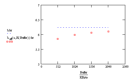
Let's
plot the probability of not overflowing the buffer for various buffer sizes.
Since we wish that probability to exceed 95%, we'll also plot a horizontal line
at 95.
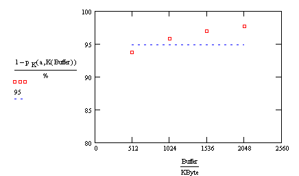
A
quick look at the graph tells us that we need to buy 1 MByte of memory with the
print buffer. With that much memory, the chance of overflowing the buffer is
just over 4%.
![]()
Now
that we picked out a printer buffer, let's look a little more closely at the
M/M/1/K system we've set up. Notice that the blocking probability, pK, depends on traffic
intensity as well as capacity. What would happen if our estimate for a was off? That could happen if we
ended up printing more or less documents per day, or if our average document
size changed significantly.
Let's
consider two possibilities. For the first, suppose we only have to print half as
many documents as we expected. For another possibility, let's see what happens
if our average document size doubles. We'll graph both of these cases, along
with our original case, in the following plot. Note that pK is plotted using a
logarithmic scale.
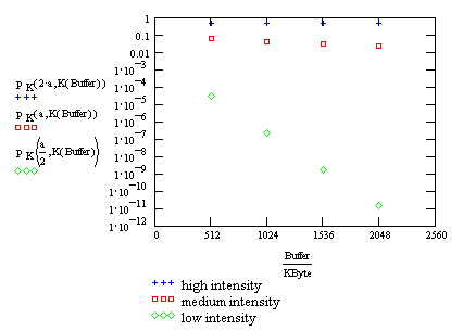
Notice
the slopes of the lines. The high intensity system is almost horizontal. That
tells us that we can't change its blocking probability much, no matter how big
a buffer we buy. The low intensity system, on the other hand, has a very steep
slope. (Remember, the y-axis is logarithmic.)
For
that system, increasing the buffer size can have a tremendous effect.
Let's
use some actual numbers to see this effect more clearly. Suppose we have a high
intensity system (because our average document size is double what we assumed
earlier.) Nearly half of the time we're waiting for the printer.
![]()
Suppose
we were to go out and buy a huge printer buffer, one with 64 MBytes of
memory.
![]()
Well,
we would manage to lower the blocking probability some. But it's doubtful that
we could justify buying 64 MBytes of memory if it only decreases that
probability by a quarter of a per cent!
How
about our the low intensity system? In that one our intensity is half because
we're only printing half as many documents in a day. Without any printer
buffer, our blocking probability is relatively low.
![]()
In
an 8-hour day, we only have to wait for the printer about 2 minutes.
![]()
Now
let's add a small printer buffer, one with only 512 KBytes of memory. With this
buffer, it takes over 3 weeks for our computer to wait 2 minutes!
![]()
We
can summarize this behavior this way: For traffic intensities less than 1,
capacity has a big effect on performance, but for traffic intensities greater
than 1, capacity has little effect.
Idle
Probability
It's
probably not that important for a printer buffer, but with some M/M/1/K queuing
systems, we're also interested in the idle probability. That's the probability
that the server is idle. We can find the probability from the same equation we
used for blocking probability. You can see the equation in the summary of
results. Here it is as a function of capacity.
![]()
Let's
plot this function for the different potential printer buffers.
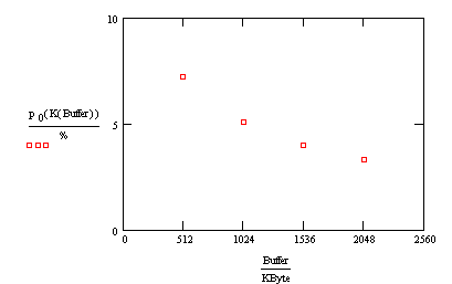
Does
the shape of this curve surprise you? The more capacity we add to the system, the
less likely we are to find the server idle. Indeed, that is the case.
Here's why. Capacity doesn't affect how much work the server is asked to do.
That depends solely on the intensity. What capacity does affect is how much
work the server can do. Without a lot of capacity, the system fills up quickly,
and potential customers are turned away. In a true M/M/1/K system these
customers are lost forever. (Of course, when a real printer buffer fills up,
subsequent documents aren't necessarily lost. By using an M/M/1/K model,
though, we've assumed that to be the case.) The lower the system capacity, the
more customers are turned away. And if a system turns away more customers, it
ultimately has less work to do and, consequently, a higher idle probability.
Effective
Arrival Rate
Another
way to consider this same result is through the effective arrival rate. Since
some customers are turned away, the system doesn't really see an arrival rate
of l.
That's how many customers try to enter. They only succeed if the system isn't
full. Here's a way to show this on a queuing system picture.
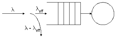
Notice
how the stream of arriving customers divides into two separate streams at the
entrance to the queue. The fraction that manage to enter the system is the same
as the fraction of the time that the system is not full. We've seen that
fraction already; it's equal to 1 - pK.
The effective arrival rate, therefore is the product of l and (1 - pK). Here's how
we can write it as a function of intensity and capacity.
![]()
As
you can see from the following graph, the effective arrival rate approaches l as our
capacity increases. The units are arrivals per hour.
There
are several other performance measures for M/M/1/K systems. They're not
particularly important for printer buffers, but they may be for other systems.
We'll look briefly at them below. To attach some real numbers, let's pick an
actual system capacity based on our initial requirements.
![]()
![]()
Average
Number in System
The
average number in the system depends only on the intensity and the capacity.
For our printer buffer, that number tells us that our system contains, on
average, just under 10 documents.
![]()
![]()
Average
System Time
We
can use Little's Law to calculate how long a customer stays in the
system. This number tells us how long it takes, on average, for a document to
finish printing. In our system that time is about an hour and a half.
![]()
![]()