The FFT: As a Set of Filter Banks
Introduction
The Fast Fourier Transform (FFT) is normally presented as an algorithm for efficiently calculating the Discrete Fourier Transform (DFT), reducing the number of required operations to O{NlogN} from the DFT’s O{N2}. In this development we will show that the FFT algorithm can be interpreted a processing the time window of the input data through a sequence of filter banks where each filter in the structure is a “Comb Filter”
The Comb Filter
A Comb Filter is a simple, one tap, feed forward, Finite Impulse Response (FIR) Filter.

If a sine wave is the input, there will be some frequencies
where the addition results in reinforcement (twice the amplitude at the peak
frequencies) and an equal number of frequencies where the two paths are exactly
out of phase resulting in no output.
Below, on the left, is a frequency response plot for a one sample
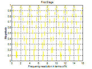
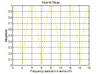
The Matlab M-file CombFFT.M shows the frequency response of each of the filters in the FFT and the resultant filter that determines the content of each “bin” for the output of the FFT. Note that the output here is the magnitude of the bin’s contents, not the complex number representing the actual FFT output. The FFT multplies by complex numbers to do the phase shift resulting in complex bins.
The “butterfly” diagram for the 16-point,
decimation-in-time, FFT algorithm illustrated in “CombFFT” is shown below.
