Linear Time-Invariant Systems (LTI)

Introduction

This section introduces the analysis of Causal, Linear, Time-invariant, Continuous systems.

• Causality: The system response depends only on inputs in the past. Excitations that will occur in the future can have no effect on the present output.
• Linearity: Superposition applies to these systems.

If x₁(t) y₁(t)
and x₂(t) y₂(t)

Then a* x₁(t) + b* x₂(t) a* y₁(t) + b* y₂(t)

Nonlinear systems are common in the real world. You will run into them in your studies of Communication Systems and Digital Signal Processing. Don’t try to apply the methods described here on non-linear systems, as they will NOT work.

• Time Invariance: These systems will behave the same now as they did yesterday. The phase of the moon has no effect. Time varying systems are also common, but we will assume an unchanging world here.
• Continuous: All variables are defined along the real line (or in the complex plane). Time progresses forward in a smooth continuous manner. System behavior can be completely described by a set of differential equations.

The input-output relationship of an LTI system can be defined in one of several ways

• Time-Domain Microscopic view: This was the first approach you used to analyze physical systems. The system behavior is described at each instant of time in terms of a set of Differential Equations and a present State.
• Time-Domain Macroscopic view: Here the system is modeled as having memory. The system output is produced as a weighted sum (integral) of its past inputs. The weighting function is called the system Impulse Response and the output is the Convolution of the past input with the Impulse response.
• Frequency Domain view: In the section on Fourier Signal Analysis the concept of the frequency domain was introduced. Now we can use the System Transfer Function to describe how the system processes the frequency domain representation of the input signal to produce the frequency domain representation of the output signal. Note that a closely related approach based on the Complex Frequency Domain (s-Domain) is covered in the section on LaPlace Transform Analysis. Both approaches are equally valid. Fourier is heavily used in Communications, while LaPlace is preferred for Feedback Controls and, in a discrete-time formulation (the Z-Transform), for Digital Signal Processing.

The Convolution Integral

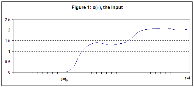
Assume that the input, x(t), to an LTI system started at time t₀ (the input was zero for all time prior to t₀₎ and has continued to the present time, t, as shown below.

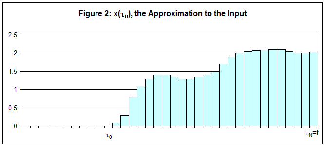
We can approximate this input as a series of rectangular pulses having the same area under the curve as shown in Figure 2.

These graphs are given in terms of the variable t, the variable t is reserved for the time of observation of the output signal. The interval from t = t₀ to t = t is divided into subintervals of width Dt each centered about an value of t_n = t₀ + n*Dt.

Now perform the following experiment. Apply a rectangular pulse of unit strength and width Dt to the input of our LTI system. Lets call the resulting output f(t, t_n).

• f(t, t_n) is the output at time t due to a rectangular pulse of unit amplitude and width Dt that occurred at time t = t_n .

The output of the system at time t due to the n^th pulse of the approximate input is then the value of the input at time t_n ,which is x(t_n), times f(t, t_n). Using superposition the total output from the system at time t is then approximated by the sum:

Multiplying and dividing each term in the sum by Dt yields:

Note that the term is the output of the time t due to a pulse of amplitude that occurred at time t = t_n . The area of this input pulse ise equal to unity. Our approximation gets better as Dt approaches zero so take the limit of y(t) as Dt 0 changing the sum to an integral.

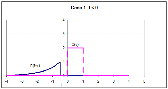
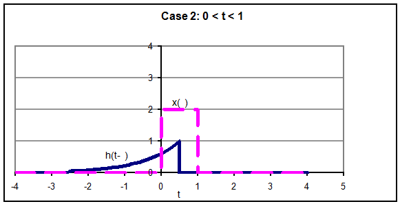
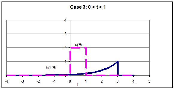
The term in the brackets becomes the output at time, t, of the system to d(t-t), a Dirac Delta function or impulse that occurred at time t . It is usually denoted as h(t, t), or since our system is time invariant simply h(t-t). This function, h(t), is called the Unit Impulse Response of the system (which happens to be the Inverse Fourier Transform of the Transfer Function, H(jw) ). The output then is given by:

or, where it is up to you to determine the limits on the integral from the nature of the two functions:

This is known as the Convolution Integral and is denoted as:

Note: The meaning of Convolution is that an LTI system can be modeled as having a memory that stores all past input. Acording to this model, the LTI system determines its output by performing a weighted sum of all past inputs using the Impulse Response as the weighting factor.

Continuous systems seldom actually function this way, but this model accurately determines the output. Many Discrete-Time LTI systems ARE built according to the Convolution model. They are called Finite Impulse Response systems since their memory has a limited capacity.

Convolution as an Operator

Commutative Law

Proof:

Let u = t - t , therefore t = t – u and

Reversing the limits is the same as multiplying by –1

Q. E. D.

Distributive Law

Proof:

Integration is a linear operator and multiplication distributes over addition

Associative Law

Proof:

Due to the convolution Law of Fourier transforms

But multiplication is Associative so

Therefore

Q. E. D.

Example Convolutions

Convolution Example 1: Simple Rectangular Functions

First flip h(t) by letting t = -t

Now shift h(-t) to the time for Case 1 by replacing (–t) with t - t

Case 2 moves the front edge of h(t-t) into x(t) so the output is the shaded area t

For all of Case 3 h(t-t) is fully within x(t) so the output is 1

In Case 4 h(t-t) is exiting x(t) so the output is [ 2 – (t-1) ]*1 or (3-t)

For all of the last Case t > 3 and there is no overlap so the output is 0

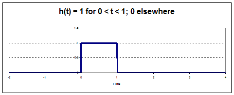
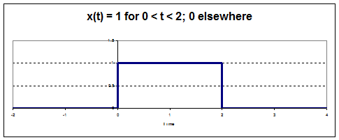
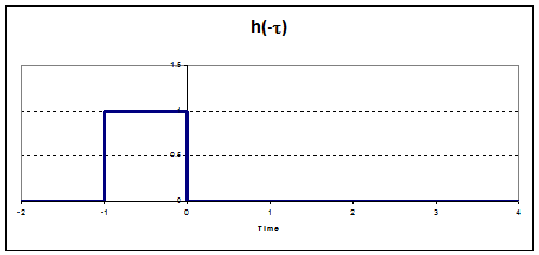
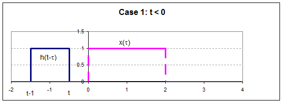
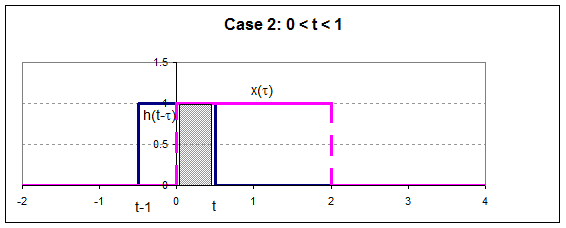
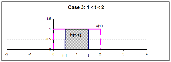
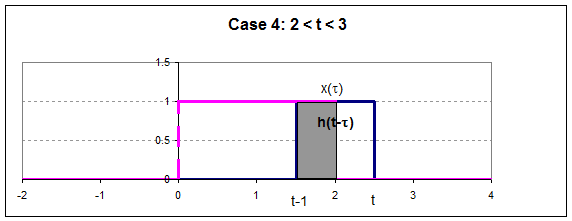
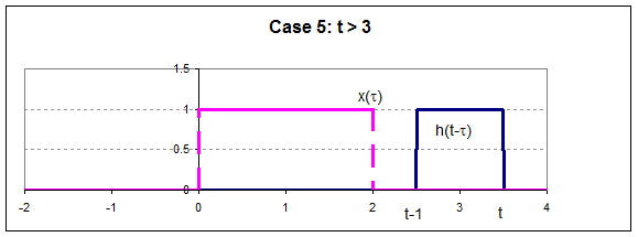
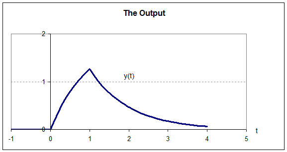
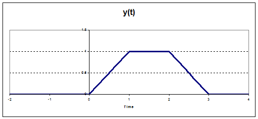So now we can plot the output, and we are done.

Convolution Example 2: A Triangular Function

The input signal x(t) is a unit rectangular pulse from t = -1 to t = 1

The system Impulse Response is triangular

Find the output,

First flip the Impulse Response by substituting t = -t

Now slide it back to start at a value of t £ -1 and plot the signal on the same chart

There is no overlap so y = 0 for t < -1

Now slide the tip of h(t-t) just past t = -1 to set up Case 2

The shaded area is the integral of the product of the two functions. And:

for 0 < t < 1

Case 3 is set up by sliding t to just past t = 1. Now the complete signal lies within the memory of the system.

Now

for 1 < t < 2

The fourth Case occurs when the back edge of h(t-t) crosses t = -1. This is when t = 2.

Now for 2 > t > 4

The last Case is when t > 4. Now there is no overlap and the output remains at zero.

Now we can plot y(t). Note that it is a continuous function. This is the normal case (the exception is when there are Impulse Functions in either the signal or h(t) ). Use this fact to check your work by comparing the values at the boundary conditions between cases.

Convolution Example 3: The RC Low Pass Filter

The input signal x(t) is a unit rectangular pulse from t = 0 to t = t₀

The circuit is:

Find the Impulse Response of the circuit using the Transfer Function:

Since it is a simple AC voltage divider

From Example 1 of the section on Fourier Transforms the inverse transform of this Transfer function is:

which looks like:

The input, v_in, is:

Now using Convolution, find the output:

Flipping h(t), sliding it to the left, t < 0, we have Case 1:

And of course y(t) = 0 for t < 0 since there is no overlap.

Case 2 is while the leading edge of h(t-t) is within the square pulse or when 0 < t < 1

Now the integral becomes:

for 0 < t < 1

Case 3 is the final case and it is good for t > 1

Now the integral becomes:

Moreover, we can now plot the output:

Review: We will next solve the same problem using methods from earlier courses.

Using Fourier Transform Analysis (Frequency Domain):

Again and

Taking the Fourier Transform of v_in(t)

The Fourier Transform of the output is then the product of this result with the Transfer function. Or:

Or,

Using a Partial Fraction Expansion,

And,

Or,

The first term is the Fourier Transform of the original input signal. Expanding the second term yields:

We can now take the Inverse Fourier Transform term by term.

Checking this out against our result using Convolution:

Case 1 (t < 0):

Case 2 (0 < t < 1):

Case 3 (t > 1):

We have the same result!

Solve the same problem once more but use Differential Equations (Microscopic Time Domain):

Remember the original circuit diagram

The Kirchoff loop equation is:

First solve the Homogeneous Equation to get the Homogeneous “Natural” solution:

Differentiating both sides of the equation and multiplying by C

The solution to this equation is of the form and substituting:

Simplifying,

or a = 1/RC

The Homogeneous Solution is therefore:

But since the voltage across the capacitor starts at 0 and,

But we want the voltage out which is:

Substituting,

where k is the constant of integration

Now we need to find the Particular Solution that is due to the Forcing Function (input)

Case 1 (t < 0): obviously, the output is again zero.

Case 2 (0 < t < 1)

We have that the original input is a constant “2” which was differentiated and became 0

The output needs to be of the form

Substituting into our original differential equation:

Or,

Since this must be true for all 0 < t < 1, B = 0 (from the t term) and from the constant term

A also is 0 so

Therefore the total solution is

but this must be zero at t = 0

for 0 < t < 1

Now for Case 3 (t > 1)

The Capacitor now discharges through the resistor from its value at t = 1.

And once again we get the same solution.