Discrete Time Systems
Introduction
y(nTs)
In our discussion of Sampling we
introduced an analog system which was equivalent to a discrete-time system.
If we simplify our notation,
![]()
![]()
and
![]()
xn yn hn
We get the discrete-time system.
![]()
![]()
Where the input, output and “pulse response” are each sequences of sampled values of the corresponding analog function.
Macroscopic Time Domain Analysis
In our Linear Systems discussion, we found that the output, y(t), of a linear system is related to its input, x(t), by the Convolution Integral,
![]() Note: the limits normally are from 0 to t since the input starts at
t=0 and the impulse response is 0 for values less than 0
Note: the limits normally are from 0 to t since the input starts at
t=0 and the impulse response is 0 for values less than 0
But, in this case,
![]() For x(t) = 0 when t
< 0 and assuming ideal sampling
For x(t) = 0 when t
< 0 and assuming ideal sampling
Therefore
![]()
Now interchanging the order of integration and summation and using the sifting property of d-functions
![]()
And using the sifting property of the delta function
![]()
Now we resample at t = n*Ts:
![]()
Again using our simplified notation, we obtain the “Convolution Sum”
![]()
Where hn is the sequence of samples of the original impulse response at the t = n*Ts
If we let the input sequence, xn, be the unit pulse at n = 0
![]()
![]() so hn
is the “Unit Pulse Response” of the discrete-time system
so hn
is the “Unit Pulse Response” of the discrete-time system
In general h(n,k) is the response at sample
time n due to a pulse that occurred at sample time k
An example discrete-time system
yn

Let xn = dn Therefore yn = { 1, a, a2, a3, …..) = an and hn = an for n ≥ 0
Note: yn = 0
for n < 0 and for stability | a| ≤ 1
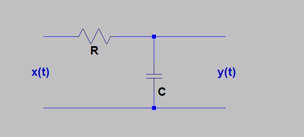
since ![]() this discrete-time system is equivalent (within a gain
factor) to the simple RC low-pass filter (“leaky bucket”) which has been used
often as an analog system example in these notes. The time Constant, RC, is:
this discrete-time system is equivalent (within a gain
factor) to the simple RC low-pass filter (“leaky bucket”) which has been used
often as an analog system example in these notes. The time Constant, RC, is:
![]()
We can now solve for the output of this system given any input through the use of the convolution sum.
Let xn be the discrete-time version of the unit step function
![]()
And let the system be initially at rest (yn = 0).
The output is given by the convolution sum as
![]() The second form is the
commutative version and is easier to use for this calculation.
The second form is the
commutative version and is easier to use for this calculation.
We have two cases:
For n < 0 all of the input values are zero and the sum is zero
For n ≥ 0 the sum becomes
![]()
This is a simple geometric series. To get a closed form without resorting to formulas pull out the first term and add/subtract an extra term
![]()
Now let p = k - 1
![]()
![]()
![]() or
or
![]() for n ≥ 0
for n ≥ 0
We therefore have our macroscopic approach to solving for the output of discrete-time systems.
Microscopic Time Domain analysis
For a microscopic analysis note how we determined hn for the example system. We actually calculated each output at time n from a knowledge of the input at time n and the “state” of the memory (or delay elements) in the system. For the example system:
![]() or
or
![]()
This is a finite difference equation which describes the example system at a moment in time. It is analogous to the differential equation:
![]()
which describes the RC low pass example in the discussion of Linear Systems.
These difference equations can be solved directly using the same techniques used to solve differential equations. As an example we will solve the same problem used in the section on discrete convolution.
![]() ; 0 < a < 1; xn is
the unit step and the system is initially at rest with yn
= 0.
; 0 < a < 1; xn is
the unit step and the system is initially at rest with yn
= 0.
Step 1: Find the homogeneous (AKA natural or transient) solution
![]()
Assume an exponential solution yn = Cn
Cn - aC(n-1) = 0
C n = aC(n-1)
or
C = a
The homogeneous solution is therefore
yn = KH * an
Step 2: Find the particular (AKA forced or steady-state) solution – we shall again use the method of undetermined coefficients
The particular solution for this problem must be of the form
yn = K0 + K1*n since the input is a constant. Therefore
y(n-1) = (K0 – K1) +K1*n
Now substituting into the difference equation for n ≥ 0
K0 + K1*n –a[(K0 – K1) +K1*n = 1
Or
[K0*(1-a) + a* K1] + [K1(1-a)]*n = 1
Therefore
K1 = 0 and K0 = 1/(1-a)
The total solution is the sum of the homogeneous and particular solutions so
yn = KH*an +1/(1-a)
but y0 = 1 so
1 = KH*a0 +1/(1-a)
Or KH = 1 – 1/(1-a) = -a/(1-a)
This makes the total solution
yn = -a(n+1)/(1-a) + 1/(1-a)
Or
yn = [1-a(n+1)]/(1-a) for n ≥ 0
Which agrees with our previous solution.